Mass Spec Alignment Example

Mass Spec Alignment Example

This tutorial shows how to take two data files and align them.

The Data Sets

The First Data Set

Raw mass spec data must be converted to a format that can be read by obi-warp. First, try to get your data into a rectilinear matrix, to look something like this:

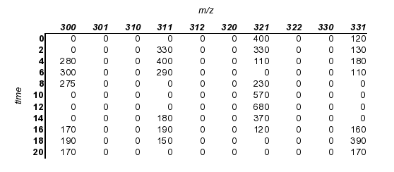
This may require that you round to the nearest m/z (the other tutorial on mass spec alignment discusses some tools for doing this)

Then, convert your data into the 'lmata' format to be read by obiwarp (an explanation of the format follows):

set1.lmata

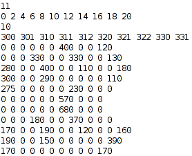
Here is an explanation of the format:

Line #	Explanation
1	number of time values (# rows in data matrix)
2	the time values
3	number of m/z values (# cols in data matrix)
4	the m/z values
5—15	An (mxn) matrix with columns being different m/z values and rows being different time values

The Second Data Set

Here is a dataset that we'd like to align to the first:

set2.lmata

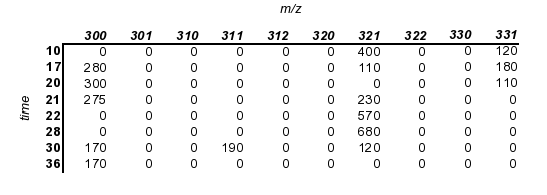
We will align this data set to the first one (obiwarp aligns along the m axis, so in this case we are aligning the times)

This is a plot of the two data sets:

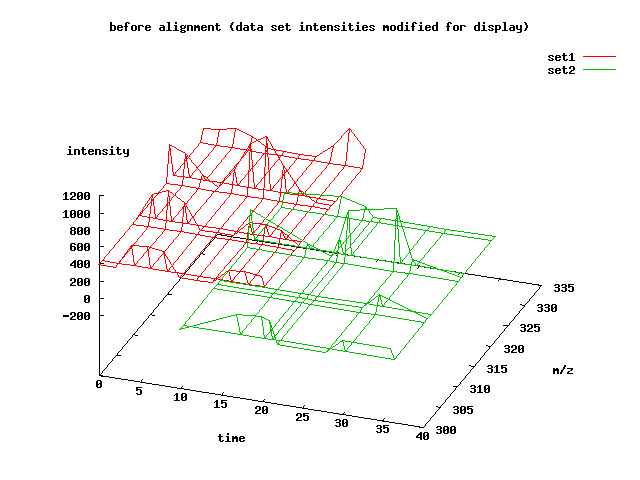
The intensity values of the sets have been adjusted so that it is easier to view them both simultaneously. Notice that the second data set has fewer time points than the first. It begins much later in time and it contains areas of compression and decompression. Most of the peaks are the same, but some are missing or slightly different than in the first data set.

Aligning the Data Sets

We can try to align them with obiwarp's default parameters:

obiwarp set1.lmata set2.lmata

This outputs the line:

0 5.38462 7.69231 8.46154 9.23077 13.8462 15.3846 20

obiwarp is outputting values for what it thinks the 8 time points should be for the second data set to bring it into the best alignment with the first data set. Basically, it's saying that the second data set should look like this:

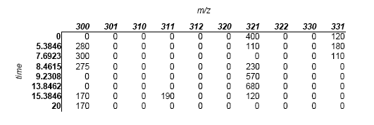
Note that only the time values have changed.

Using obiwarp's default parameters, we see that the result is in the ballpark, but not perfect:

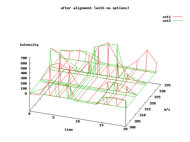
The resulting alignment can be somewhat dependent on the options given to obiwarp, especially if the strength of the overlapping signals are not strong.

Probably the two most useful parameters to play around with are the gap penalty and the response. The gap penalty takes two values, an initiation penalty and an elongation penalty. Essentially, large gap penalties become more important the noisier the data. Type obiwarp --help long to see the default gap penalties for each different score function. The response can be thought of as the percentage of inflection points to use in creating an alignment. You usually won't go wrong keeping this value close to 100. 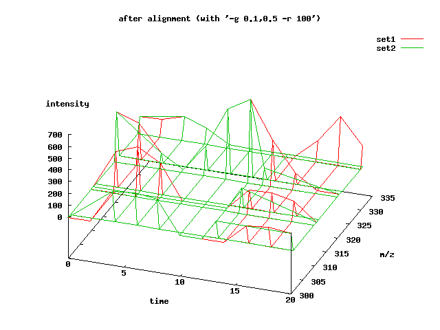Here, we relax the gap penalty a bit and increase the response to 100%:

 obiwarp -r 100 -g 0.1,0.5 set1.lmata set2.lmata

The result is a better alignment:

the other tutorial on mass spec alignment discusses a more sophisticated method for measuring alignment quality than just plotting the data.

Plotting Tools

The simple script lmata_to_gnuplot_dat.rb can be used to transform a .lmata file into a .dat file that gnuplot can read. Executing the script with no parameters (./lmata_to_gnuplot_dat.rb) will also suggest some gnuplot commands that can be used to plot the .dat files. The commands can be included in a file (e.g., 'mycommands.txt') and executed by typing gnuplot mycommands.txt.